Building a Complete Machine Learning Pipeline using scikit-learn
Learn how to build an end-to-end ML pipeline from data preprocessing to model deployment using scikit-learn

Introduction
In this comprehensive tutorial, we'll build a production-ready machine learning pipeline from scratch using scikit-learn. You'll learn how to:
- Load and explore datasets
- Handle missing data and outliers
- Encode categorical variables
- Scale numerical features
- Build and evaluate models
- Create reusable pipelines
- Save and deploy models
What you'll build:
A complete ML pipeline that predicts house prices using the California Housing dataset, with proper data preprocessing, feature engineering, model training, and evaluation.
What is a Machine Learning Pipeline?
A machine learning pipeline is an automated workflow that chains together multiple data processing and modeling steps. Instead of manually applying transformations, you create a pipeline that:
- Ensures consistency between training and production
- Prevents data leakage by applying transformations in the right order
- Makes code reusable and maintainable
- Simplifies deployment with a single serialized object
Pipeline Benefits:
Think of it like a factory assembly line - raw materials (data) go in one end, and a finished product (predictions) comes out the other, with quality checks at each stage.
Prerequisites
Tech Stack
Project Structure
ml-pipeline/
├── data/
│   ├── raw/                  # Original datasets
│   └── processed/            # Cleaned datasets
├── notebooks/
│   └── exploration.ipynb     # EDA notebook
├── src/
│   ├── data_loader.py        # Data loading utilities
│   ├── preprocessing.py      # Feature engineering
│   ├── pipeline.py           # ML pipeline definition
│   ├── train.py              # Training script
│   ├── analysis.py           # Model interpretation
│   ├── predict.py            # Prediction utilities
│   └── monitoring.py         # Production monitoring
├── tests/
│   └── test_pipeline.py      # Unit tests
├── models/
│   └── model.pkl             # Saved model
├── app.py                    # Flask API
├── test_api.py               # API testing script
├── Dockerfile                # Docker configuration
├── docker-compose.yml        # Docker Compose config
├── requirements.txt          # Python dependencies
└── README.md                 # Project documentation
Step 1: Setup and Installation
- 1
Create a virtual environment.
- 2
Install dependencies.
- 3
Set up project structure.
Create Virtual Environment
# Create project directory
mkdir ml-pipeline ml-pipeline\data ml-pipeline\notebooks ml-pipeline\src ml-pipeline\models ml-pipeline\tests
cd ml-pipeline

# Create virtual environment
python -m venv venv

# Activate virtual environment
source venv/bin/activate  # Linux/Mac
venv\Scripts\activate  # Windows
Install Dependencies
pandas==2.3.3
numpy==2.3.3
scikit-learn==1.7.2
matplotlib==3.10.6
seaborn==0.13.2
jupyter==1.1.1
joblib==1.5.2
Flask==3.1.2
pytest==8.4.2
gunicorn==23.0.0pip install -r requirements.txtStep 2: Load and Explore the Dataset
We'll use the California Housing dataset, which contains information about houses in California districts.
import pandas as pd
import numpy as np
from sklearn.datasets import fetch_california_housing
from sklearn.model_selection import train_test_split

def load_data():
  """Load California Housing dataset"""
  housing = fetch_california_housing(as_frame=True)
  df = housing.frame

  print(f"Dataset shape: {df.shape}")
  print(f"\nFeatures: {housing.feature_names}")
  print(f"\nTarget: {housing.target_names}")

  return df

def split_data(df, test_size=0.2, random_state=42):
  """Split data into train and test sets"""
  X = df.drop('MedHouseVal', axis=1)
  y = df['MedHouseVal']

  X_train, X_test, y_train, y_test = train_test_split(
      X, y, test_size=test_size, random_state=random_state
  )

  print(f"\nTraining set size: {X_train.shape[0]}")
  print(f"Test set size: {X_test.shape[0]}")

  return X_train, X_test, y_train, y_test

if __name__ == "__main__":
  df = load_data()
  print(df.head())
  print(f"\n{df.describe()}")
  print(f"\n{df.info()}")
Test the data loader:
Run the script to verify data loads correctly:
python src/data_loader.pyCalifornia Housing Dataset Features:
- MedInc: Median income in block group
- HouseAge: Median house age in block group
- AveRooms: Average number of rooms per household
- AveBedrms: Average number of bedrooms per household
- Population: Block group population
- AveOccup: Average number of household members
- Latitude: Block group latitude
- Longitude: Block group longitude
- MedHouseVal: Median house value (target variable, in $100,000s)
Step 3: Exploratory Data Analysis
Let's visualize and understand our data.
import sys, os
import matplotlib.pyplot as plt
import seaborn as sns

sys.path.append(os.path.abspath(os.path.join('..')))
from src.data_loader import load_data

sns.set_style("whitegrid")
plt.rcParams['figure.figsize'] = (12, 6)

# Load data
df = load_data()

# Check for missing values
print("Missing values per column:")
print(df.isnull().sum())

# Distribution of target variable
plt.figure(figsize=(10, 5))
plt.subplot(1, 2, 1)
df['MedHouseVal'].hist(bins=50, edgecolor='black')
plt.xlabel('Median House Value ($100k)')
plt.ylabel('Frequency')
plt.title('Distribution of House Prices')

plt.subplot(1, 2, 2)
df.boxplot(column='MedHouseVal')
plt.ylabel('Median House Value ($100k)')
plt.title('Boxplot of House Prices')
plt.tight_layout()
plt.show()

# Correlation matrix
plt.figure(figsize=(12, 8))
correlation_matrix = df.corr()
sns.heatmap(correlation_matrix, annot=True, cmap='coolwarm', center=0)
plt.title('Feature Correlation Matrix')
plt.tight_layout()
plt.show()

# Geographic scatter plot
plt.figure(figsize=(10, 7))
scatter = plt.scatter(
  df['Longitude'],
  df['Latitude'],
  c=df['MedHouseVal'],
  cmap='viridis',
  alpha=0.4,
  s=10
)
plt.colorbar(scatter, label='Median House Value ($100k)')
plt.xlabel('Longitude')
plt.ylabel('Latitude')
plt.title('California Housing Prices by Location')
plt.show()

# Feature distributions
fig, axes = plt.subplots(3, 3, figsize=(15, 12))
axes = axes.ravel()

for idx, col in enumerate(df.columns):
  axes[idx].hist(df[col], bins=50, edgecolor='black')
  axes[idx].set_title(col)
  axes[idx].set_xlabel('Value')
  axes[idx].set_ylabel('Frequency')

plt.tight_layout()
plt.show()
Run the exploration notebook:
Or run as a Python script to see the visualizations. The correlation heatmap should show strong positive correlation between MedInc and MedHouseVal (~0.69).
jupyter notebook notebooks/exploration.ipynbDataset shape: (20640, 9)
Features: ['MedInc', 'HouseAge', 'AveRooms', 'AveBedrms', 'Population', 'AveOccup', 'Latitude', 'Longitude']
Target: ['MedHouseVal']
Missing values per column:
MedInc 0
HouseAge 0
AveRooms 0
AveBedrms 0
Population 0
AveOccup 0
Latitude 0
Longitude 0
MedHouseVal 0
dtype: int64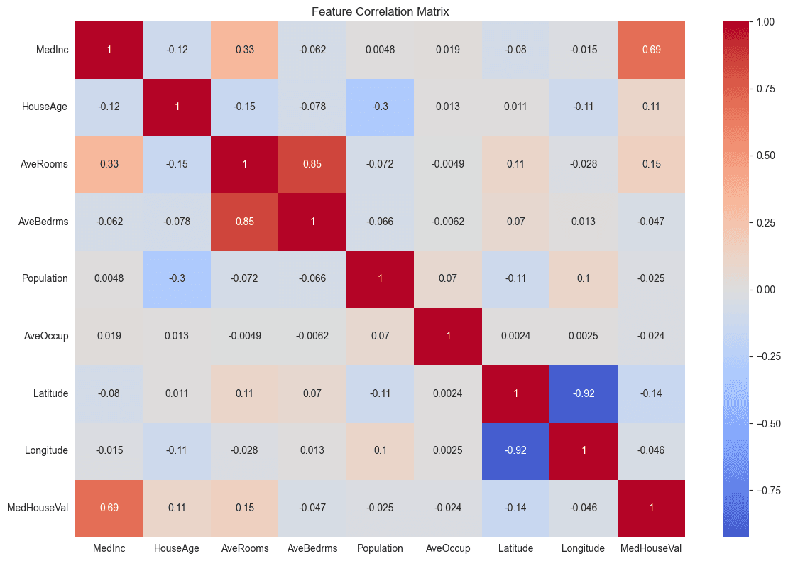
Feature Correlation Matrix

Distribution of House Prices
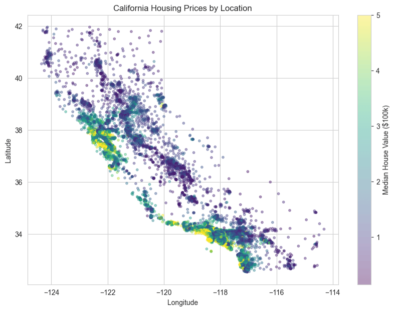
House value by location
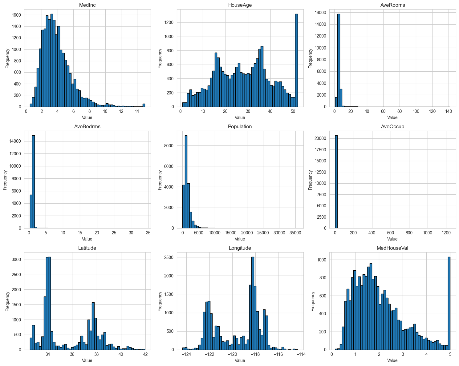
Distribution of each individual feature
Key Insights from EDA:
- No missing values in the dataset
- House values range from $15k to $500k
- Strong correlation between median income and house value
- Geographic location significantly impacts prices (coastal areas are more expensive)
- Some features are skewed and may benefit from transformation
Step 4: Feature Engineering
Create new features that might improve model performance.
import numpy as np
import pandas as pd
from sklearn.base import BaseEstimator, TransformerMixin

class FeatureEngineer(BaseEstimator, TransformerMixin):
  """Custom transformer for feature engineering"""

  def __init__(self, add_bedrooms_per_room=True):
      self.add_bedrooms_per_room = add_bedrooms_per_room

  def fit(self, X, y=None):
      return self

  def transform(self, X):
      """Create new features"""
      X = X.copy()

      # Rooms per household
      X['rooms_per_household'] = X['AveRooms'] / X['AveOccup']

      # Bedrooms ratio
      if self.add_bedrooms_per_room:
          X['bedrooms_per_room'] = X['AveBedrms'] / X['AveRooms']

      # Population per household
      X['population_per_household'] = X['Population'] / X['AveOccup']

      return X

class OutlierRemover(BaseEstimator, TransformerMixin):
  """Remove outliers using IQR method"""

  def __init__(self, factor=1.5):
      self.factor = factor
      self.bounds = {}

  def fit(self, X, y=None):
      """Calculate bounds for each feature"""
      for col in X.columns:
          Q1 = X[col].quantile(0.25)
          Q3 = X[col].quantile(0.75)
          IQR = Q3 - Q1

          lower_bound = Q1 - self.factor * IQR
          upper_bound = Q3 + self.factor * IQR

          self.bounds[col] = (lower_bound, upper_bound)

      return self

  def transform(self, X):
      """Clip outliers to bounds"""
      X = X.copy()

      for col, (lower, upper) in self.bounds.items():
          X[col] = X[col].clip(lower, upper)

      return X

if __name__ == "__main__":
  from data_loader import load_data, split_data

  df = load_data()
  X_train, X_test, y_train, y_test = split_data(df)

  # Test feature engineering
  fe = FeatureEngineer()
  X_train_fe = fe.fit_transform(X_train)

  print("Original features:", X_train.shape[1])
  print("After feature engineering:", X_train_fe.shape[1])
  print("\nNew features:")
  print(X_train_fe[['rooms_per_household', 'bedrooms_per_room',
                     'population_per_household']].head())
Test feature engineering:
python src/preprocessing.pyDataset shape: (20640, 9)
Features: ['MedInc', 'HouseAge', 'AveRooms', 'AveBedrms', 'Population', 'AveOccup', 'Latitude', 'Longitude']
Target: ['MedHouseVal']
Training set size: 16512
Test set size: 4128
Original features: 8
After feature engineering: 11
New features:
rooms_per_household bedrooms_per_room population_per_household
14196 1.359130 0.200576 623.0
8267 2.573820 0.232703 756.0
17445 2.073224 0.174486 336.0
14265 1.002116 0.258269 355.0
2271 2.725400 0.180940 380.0Step 5: Build the ML Pipeline
Now let's create a complete pipeline that handles all preprocessing and modeling.
from sklearn.pipeline import Pipeline
from sklearn.preprocessing import StandardScaler
from sklearn.impute import SimpleImputer
from sklearn.compose import ColumnTransformer
from sklearn.linear_model import LinearRegression, Ridge, Lasso
from sklearn.ensemble import RandomForestRegressor, GradientBoostingRegressor
from sklearn.model_selection import cross_val_score
import numpy as np

from src.preprocessing import FeatureEngineer, OutlierRemover

def create_preprocessing_pipeline():
  """Create preprocessing pipeline"""

  preprocessing_pipeline = Pipeline([
      ('feature_engineer', FeatureEngineer(add_bedrooms_per_room=True)),
      ('outlier_remover', OutlierRemover(factor=1.5)),
      ('scaler', StandardScaler())
  ])

  return preprocessing_pipeline

def create_full_pipeline(model_type='random_forest'):
  """Create complete pipeline with preprocessing and model"""

  # Preprocessing
  preprocessing = create_preprocessing_pipeline()

  # Model selection
  models = {
      'linear': LinearRegression(),
      'ridge': Ridge(alpha=1.0),
      'lasso': Lasso(alpha=0.1),
      'random_forest': RandomForestRegressor(
          n_estimators=100,
          max_depth=15,
          min_samples_split=5,
          random_state=42,
          n_jobs=-1
      ),
      'gradient_boosting': GradientBoostingRegressor(
          n_estimators=100,
          learning_rate=0.1,
          max_depth=5,
          random_state=42
      )
  }

  if model_type not in models:
      raise ValueError(f"Model type must be one of {list(models.keys())}")

  # Complete pipeline
  full_pipeline = Pipeline([
      ('preprocessing', preprocessing),
      ('model', models[model_type])
  ])

  return full_pipeline

def evaluate_pipeline(pipeline, X_train, y_train, cv=5):
  """Evaluate pipeline using cross-validation"""

  # Cross-validation scores
  cv_scores = cross_val_score(
      pipeline, X_train, y_train,
      cv=cv,
      scoring='neg_root_mean_squared_error',
      n_jobs=-1
  )

  rmse_scores = -cv_scores

  print(f"Cross-Validation RMSE Scores: {rmse_scores}")
  print(f"Mean RMSE: {rmse_scores.mean():.4f}")
  print(f"Std RMSE: {rmse_scores.std():.4f}")

  return rmse_scores

if __name__ == "__main__":
  from src.data_loader import load_data, split_data

  # Load data
  df = load_data()
  X_train, X_test, y_train, y_test = split_data(df)

  # Test different models
  models = ['linear', 'ridge', 'random_forest', 'gradient_boosting']

  results = {}
  for model_type in models:
      print(f"\n{'='*50}")
      print(f"Evaluating {model_type.upper()} model")
      print('='*50)

      pipeline = create_full_pipeline(model_type)
      scores = evaluate_pipeline(pipeline, X_train, y_train)
      results[model_type] = scores.mean()

  # Best model
  best_model = min(results.items(), key=lambda x: x[1])
  print(f"\n{'='*50}")
  print(f"Best Model: {best_model[0].upper()}")
  print(f"RMSE: {best_model[1]:.4f}")
  print('='*50)
Test the pipeline:
python -m src.pipelineDataset shape: (20640, 9)
Features: ['MedInc', 'HouseAge', 'AveRooms', 'AveBedrms', 'Population', 'AveOccup', 'Latitude', 'Longitude']
Target: ['MedHouseVal']
Training set size: 16512
Test set size: 4128
==================================================
Evaluating LINEAR model
==================================================
Cross-Validation RMSE Scores: [0.65081613 0.63001644 0.64790608 0.63324737 0.66694957]
Mean RMSE: 0.6458
Std RMSE: 0.0133
==================================================
Evaluating RIDGE model
==================================================
Cross-Validation RMSE Scores: [0.65081595 0.63002266 0.64791384 0.63323854 0.66693872]
Mean RMSE: 0.6458
Std RMSE: 0.0133
==================================================
Evaluating RANDOM_FOREST model
==================================================
Cross-Validation RMSE Scores: [0.51803625 0.52211652 0.5110684 0.51612053 0.51936622]
Mean RMSE: 0.5173
Std RMSE: 0.0037
==================================================
Evaluating GRADIENT_BOOSTING model
==================================================
Cross-Validation RMSE Scores: [0.48380639 0.49581548 0.48830646 0.48626087 0.49890963]
Mean RMSE: 0.4906
Std RMSE: 0.0058
==================================================
Best Model: GRADIENT_BOOSTING
RMSE: 0.4906
==================================================Step 6: Hyperparameter Tuning
Let's optimize our best model using grid search.
import sys, os
sys.path.append(os.path.dirname(os.path.dirname(os.path.abspath(__file__))))
from sklearn.model_selection import GridSearchCV
from sklearn.metrics import mean_squared_error, r2_score, mean_absolute_error
import joblib
import numpy as np

from src.pipeline import create_full_pipeline
from src.data_loader import load_data, split_data

def tune_hyperparameters(X_train, y_train, model_type='random_forest'):
  """Perform grid search for hyperparameter tuning"""

  # Create base pipeline
  pipeline = create_full_pipeline(model_type)

  # Define parameter grid
  if model_type == 'random_forest':
      param_grid = {
          'model__n_estimators': [50, 100, 200],
          'model__max_depth': [10, 15, 20, None],
          'model__min_samples_split': [2, 5, 10],
          'model__min_samples_leaf': [1, 2, 4]
      }
  elif model_type == 'gradient_boosting':
      param_grid = {
          'model__n_estimators': [50, 100, 200],
          'model__learning_rate': [0.01, 0.1, 0.2],
          'model__max_depth': [3, 5, 7],
          'model__subsample': [0.8, 1.0]
      }
  elif model_type == 'ridge':
      param_grid = {
          'model__alpha': [0.01, 0.1, 1.0, 10.0, 100.0]
      }
  else:
      raise ValueError(f"No parameter grid defined for {model_type}")

  # Grid search
  grid_search = GridSearchCV(
      pipeline,
      param_grid,
      cv=5,
      scoring='neg_root_mean_squared_error',
      n_jobs=-1,
      verbose=2
  )

  print(f"\nStarting grid search for {model_type}...")
  print(f"Parameter grid: {param_grid}")

  grid_search.fit(X_train, y_train)

  print(f"\nBest parameters: {grid_search.best_params_}")
  print(f"Best cross-validation RMSE: {-grid_search.best_score_:.4f}")

  return grid_search.best_estimator_

def evaluate_model(model, X_test, y_test):
  """Evaluate model on test set"""

  # Predictions
  y_pred = model.predict(X_test)

  # Metrics
  rmse = np.sqrt(mean_squared_error(y_test, y_pred))
  mae = mean_absolute_error(y_test, y_pred)
  r2 = r2_score(y_test, y_pred)

  print(f"\n{'='*50}")
  print("TEST SET EVALUATION")
  print('='*50)
  print(f"RMSE: {rmse:.4f}")
  print(f"MAE: {mae:.4f}")
  print(f"R² Score: {r2:.4f}")
  print('='*50)

  return {'rmse': rmse, 'mae': mae, 'r2': r2}

def save_model(model, filepath='models/model.pkl'):
  """Save trained model to disk"""
  joblib.dump(model, filepath)
  print(f"\nModel saved to {filepath}")

def load_model(filepath='models/model.pkl'):
  """Load model from disk"""
  model = joblib.load(filepath)
  print(f"\nModel loaded from {filepath}")
  return model

def train_final_model():
  """Complete training workflow"""

  # Load data
  print("Loading data...")
  df = load_data()
  X_train, X_test, y_train, y_test = split_data(df)

  # Tune hyperparameters
  print("\nTuning hyperparameters...")
  best_model = tune_hyperparameters(X_train, y_train, model_type='random_forest')

  # Evaluate on test set
  print("\nEvaluating on test set...")
  metrics = evaluate_model(best_model, X_test, y_test)

  # Save model
  save_model(best_model)

  return best_model, metrics

if __name__ == "__main__":
  model, metrics = train_final_model()
Run training:
python src/train.pyThis will:
- Perform grid search (takes some time)
- Evaluate on test set
- Save the model to 'models/model.pkl'
Best parameters: {'model__max_depth': None, 'model__min_samples_leaf': 2, 'model__min_samples_split': 2, 'model__n_estimators': 200}
Best cross-validation RMSE: 0.5133

Evaluating on test set...

==================================================
TEST SET EVALUATION
==================================================
RMSE: 0.5042
MAE: 0.3297
R² Score: 0.8060
==================================================

Model saved to models/model.pkl
Step 7: Model Interpretation
Let's analyze feature importance and model predictions.
import matplotlib.pyplot as plt
import seaborn as sns
import numpy as np
import pandas as pd
def plot_feature_importance(model, feature_names, top_n=15):
"""Plot feature importance for tree-based models"""
# Get feature importances
if hasattr(model.named_steps['model'], 'feature_importances_'):
importances = model.named_steps['model'].feature_importances_
else:
print("Model does not have feature_importances_ attribute")
return
# Create dataframe
feature_importance_df = pd.DataFrame({
'feature': feature_names,
'importance': importances
}).sort_values('importance', ascending=False).head(top_n)
# Plot
plt.figure(figsize=(10, 6))
sns.barplot(data=feature_importance_df, x='importance', y='feature', palette='viridis')
plt.title(f'Top {top_n} Most Important Features')
plt.xlabel('Importance')
plt.ylabel('Feature')
plt.tight_layout()
plt.show()
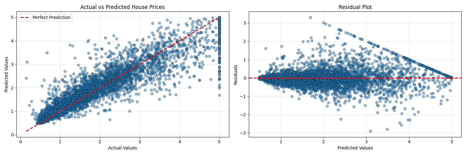
def plot_predictions(y_test, y_pred):
"""Plot actual vs predicted values"""
fig, axes = plt.subplots(1, 2, figsize=(15, 5))
# Scatter plot
axes[0].scatter(y_test, y_pred, alpha=0.5, edgecolors='k', linewidth=0.5)
axes[0].plot([y_test.min(), y_test.max()],
[y_test.min(), y_test.max()],
'r--', lw=2, label='Perfect Prediction')
axes[0].set_xlabel('Actual Values')
axes[0].set_ylabel('Predicted Values')
axes[0].set_title('Actual vs Predicted House Prices')
axes[0].legend()
axes[0].grid(True, alpha=0.3)
# Residuals plot
residuals = y_test - y_pred
axes[1].scatter(y_pred, residuals, alpha=0.5, edgecolors='k', linewidth=0.5)
axes[1].axhline(y=0, color='r', linestyle='--', lw=2)
axes[1].set_xlabel('Predicted Values')
axes[1].set_ylabel('Residuals')
axes[1].set_title('Residual Plot')
axes[1].grid(True, alpha=0.3)
plt.tight_layout()
plt.show()
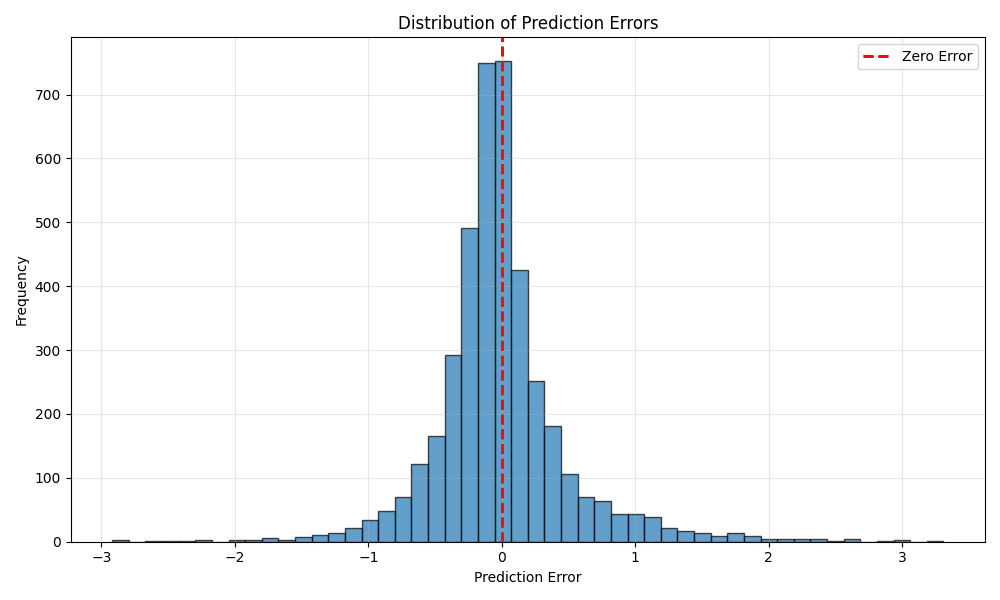
def plot_error_distribution(y_test, y_pred):
"""Plot distribution of prediction errors"""
errors = y_test - y_pred
plt.figure(figsize=(10, 6))
plt.hist(errors, bins=50, edgecolor='black', alpha=0.7)
plt.axvline(x=0, color='r', linestyle='--', linewidth=2, label='Zero Error')
plt.xlabel('Prediction Error')
plt.ylabel('Frequency')
plt.title('Distribution of Prediction Errors')
plt.legend()
plt.grid(True, alpha=0.3)
plt.tight_layout()
plt.show()
print(f"\nError Statistics:")
print(f"Mean Error: {errors.mean():.4f}")
print(f"Std Error: {errors.std():.4f}")
print(f"Min Error: {errors.min():.4f}")
print(f"Max Error: {errors.max():.4f}")
if __name__ == "__main__":
from data_loader import load_data, split_data
from train import load_model
from preprocessing import FeatureEngineer
# Load data and model
df = load_data()
X_train, X_test, y_train, y_test = split_data(df)
model = load_model()
# Get feature names after engineering
fe = FeatureEngineer()
X_train_fe = fe.fit_transform(X_train)
feature_names = X_train_fe.columns.tolist()
# Make predictions
y_pred = model.predict(X_test)
# Visualizations
plot_feature_importance(model, feature_names)
plot_predictions(y_test, y_pred)
plot_error_distribution(y_test, y_pred)Analyze the model:
python src/analysis.pyThis will generate three visualizations:
- Feature Importance Plot - Shows MedInc is typically the most important feature
- Residual Plot - Should show random scatter around zero (no patterns)
- Actual vs Predicted Plot - Should show points clustered around the diagonal line
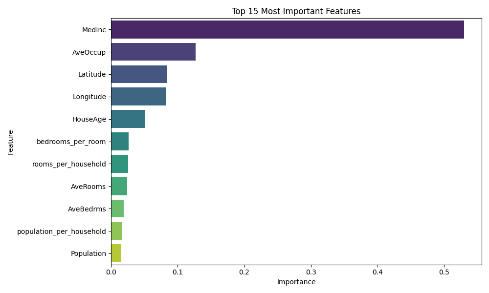
Feature Importance
Residual Plot
Actual vs Predicted Plot
Step 8: Making Predictions
Create a simple interface for making predictions on new data.
import pandas as pd
import numpy as np
from train import load_model

def predict_house_price(model, house_data):
  """
  Predict house price for new data

  Parameters:
  -----------
  model : sklearn pipeline
      Trained model pipeline
  house_data : dict or pd.DataFrame
      House features

  Returns:
  --------
  float : Predicted house price
  """

  # Convert dict to dataframe if needed
  if isinstance(house_data, dict):
      house_data = pd.DataFrame([house_data])

  # Make prediction
  prediction = model.predict(house_data)

  # Convert from $100k units to actual dollars
  price_in_dollars = prediction[0] * 100000

  return price_in_dollars

def predict_batch(model, csv_path):
  """Make predictions for multiple houses from CSV"""

  # Load data
  data = pd.read_csv(csv_path)

  # Make predictions
  predictions = model.predict(data)

  # Add predictions to dataframe
  data['PredictedPrice'] = predictions * 100000

  return data

# Example usage
if __name__ == "__main__":
  # Load model
  model = load_model()

# Example usage
if __name__ == "__main__":
  # Load model
  model = load_model()

  # Example house data
  example_house = {
      'MedInc': 8.3252,
      'HouseAge': 41.0,
      'AveRooms': 6.984127,
      'AveBedrms': 1.023810,
      'Population': 322.0,
      'AveOccup': 2.555556,
      'Latitude': 37.88,
      'Longitude': -122.23
  }

  # Predict
  predicted_price = predict_house_price(model, example_house)

  print(f"\nHouse Features:")
  for key, value in example_house.items():
      print(f"  {key}: {value}")

  print(f"\nPredicted Price: ${predicted_price:,.2f}")
Test predictions:
python src/predict.pyModel loaded from models/model.pkl
House Features:
MedInc: 8.3252
HouseAge: 41.0
AveRooms: 6.984127
AveBedrms: 1.02381
Population: 322.0
AveOccup: 2.555556
Latitude: 37.88
Longitude: -122.23
Predicted Price: $435,519.72Step 9: Model Deployment (Flask API)
Create a simple REST API to serve predictions.
from flask import Flask, request, jsonify
import pandas as pd
from src.train import load_model

# Initialize Flask app
app = Flask(__name__)

# Load model at startup
model = load_model('models/model.pkl')

@app.route('/')
def home():
  return jsonify({
      'message': 'House Price Prediction API',
      'endpoints': {
          '/predict': 'POST - Predict single house price',
          '/predict_batch': 'POST - Predict multiple house prices',
          '/health': 'GET - Check API health'
      }
  })

@app.route('/health')
def health():
  return jsonify({'status': 'healthy'})

@app.route('/predict', methods=['POST'])
def predict():
  """Predict house price for single input"""
  try:
      # Get data from request
      data = request.get_json()

      # Validate required fields
      required_fields = ['MedInc', 'HouseAge', 'AveRooms', 'AveBedrms',
                        'Population', 'AveOccup', 'Latitude', 'Longitude']

      missing_fields = [field for field in required_fields if field not in data]
      if missing_fields:
          return jsonify({
              'error': f'Missing required fields: {missing_fields}'
          }), 400

      # Create dataframe
      df = pd.DataFrame([data])

      # Make prediction
      prediction = model.predict(df)[0]
      price_in_dollars = prediction * 100000

      return jsonify({
          'predicted_price': round(price_in_dollars, 2),
          'price_range': f'${price_in_dollars:,.0f}',
          'input_data': data
      })

  except Exception as e:
      return jsonify({'error': str(e)}), 500

@app.route('/predict_batch', methods=['POST'])
def predict_batch():
  """Predict house prices for multiple inputs"""
  try:
      # Get data from request
      data = request.get_json()

      if not isinstance(data, list):
          return jsonify({
              'error': 'Input must be a list of house data objects'
          }), 400

      # Create dataframe
      df = pd.DataFrame(data)

      # Make predictions
      predictions = model.predict(df)
      prices = (predictions * 100000).tolist()

      # Format results
      results = [
          {
              'input': house,
              'predicted_price': round(price, 2),
              'price_range': f'${price:,.0f}'
          }
          for house, price in zip(data, prices)
      ]

      return jsonify({
          'predictions': results,
          'count': len(results)
      })

  except Exception as e:
      return jsonify({'error': str(e)}), 500

if __name__ == '__main__':
  app.run(debug=True, host='0.0.0.0', port=5000)
Start the API server:
python app.pyTest the API
import requests
import json

# API endpoint
url = 'http://localhost:5000/predict'

# Example house data
house_data = {
  'MedInc': 8.3252,
  'HouseAge': 41.0,
  'AveRooms': 6.984127,
  'AveBedrms': 1.023810,
  'Population': 322.0,
  'AveOccup': 2.555556,
  'Latitude': 37.88,
  'Longitude': -122.23
}

# Make request
response = requests.post(url, json=house_data)

# Print result
print(json.dumps(response.json(), indent=2))
Test with Python:
# In a new terminal (keep Flask running)
python test_api.py
Expected output:
{
"input_data": {
  "AveBedrms": 1.02381,
  "AveOccup": 2.555556,
  "AveRooms": 6.984127,
  "HouseAge": 41.0,
  "Latitude": 37.88,
  "Longitude": -122.23,
  "MedInc": 8.3252,
  "Population": 322.0
},
"predicted_price": 435519.72,
"price_range": "$435,520"
}
Step 10: Docker Deployment
Containerize the application for easy deployment.
FROM python:3.11-slim

# Set working directory
WORKDIR /app

# Copy requirements first (for caching)
COPY requirements.txt .

# Install dependencies
RUN pip install --no-cache-dir -r requirements.txt

# Copy application code
COPY . .

# Expose port
EXPOSE 5000

# Set environment variables
ENV PYTHONUNBUFFERED=1

# Run the application
CMD ["gunicorn", "-w", "4", "-b", "0.0.0.0:5000", "app:app"]version: '3.8'
services:
ml-api:
build: .
ports:
- "5000:5000"
volumes:
- ./models:/app/models
- ./data:/app/data
environment:
- FLASK_ENV=production
restart: unless-stopped# Build and run with Docker
docker build -t house-price-predictor .
docker run -p 5000:5000 house-price-predictor
# Or use docker-compose
docker-compose up -dPerformance Optimization Tips
Common Issues and Solutions
Testing Your Pipeline
import pytest
import numpy as np
import pandas as pd
from sklearn.datasets import fetch_california_housing

from src.pipeline import create_full_pipeline, create_preprocessing_pipeline
from src.preprocessing import FeatureEngineer, OutlierRemover
from src.data_loader import load_data, split_data

class TestPreprocessing:
  """Test preprocessing components"""

  def test_feature_engineer(self):
      """Test feature engineering transformer"""
      # Create sample data
      X = pd.DataFrame({
          'AveRooms': [6.0, 7.0],
          'AveBedrms': [1.0, 1.2],
          'AveOccup': [3.0, 2.5],
          'Population': [300, 250]
      })

      fe = FeatureEngineer()
      X_transformed = fe.fit_transform(X)

      # Check new features exist
      assert 'rooms_per_household' in X_transformed.columns
      assert 'bedrooms_per_room' in X_transformed.columns
      assert 'population_per_household' in X_transformed.columns

      # Check calculations
      assert X_transformed['rooms_per_household'].iloc[0] == 6.0 / 3.0

  def test_outlier_remover(self):
      """Test outlier removal"""
      X = pd.DataFrame({
          'feature1': [1, 2, 3, 4, 100]  # 100 is an outlier
      })

      remover = OutlierRemover(factor=1.5)
      X_transformed = remover.fit_transform(X)

      # Check that outlier was clipped
      assert X_transformed['feature1'].max() < 100

class TestPipeline:
  """Test complete pipeline"""

  def test_pipeline_creation(self):
      """Test pipeline can be created"""
      pipeline = create_full_pipeline('random_forest')
      assert pipeline is not None
      assert 'preprocessing' in pipeline.named_steps
      assert 'model' in pipeline.named_steps

  def test_pipeline_fit_predict(self):
      """Test pipeline can fit and predict"""
      # Load data
      df = load_data()
      X_train, X_test, y_train, y_test = split_data(df, test_size=0.2)

      # Create and train pipeline
      pipeline = create_full_pipeline('random_forest')
      pipeline.fit(X_train, y_train)

      # Make predictions
      predictions = pipeline.predict(X_test)

      # Check predictions
      assert len(predictions) == len(X_test)
      assert predictions.dtype == np.float64
      assert np.all(predictions > 0)  # House prices should be positive

  def test_pipeline_score(self):
      """Test pipeline produces reasonable scores"""
      df = load_data()
      X_train, X_test, y_train, y_test = split_data(df, test_size=0.2)

      pipeline = create_full_pipeline('random_forest')
      pipeline.fit(X_train, y_train)

      score = pipeline.score(X_test, y_test)

      # R² score should be positive and reasonable
      assert score > 0.5  # At least moderate fit
      assert score < 1.0  # Not perfect (would indicate overfitting)

class TestDataLoader:
  """Test data loading utilities"""

  def test_load_data(self):
      """Test data loading"""
      df = load_data()

      assert isinstance(df, pd.DataFrame)
      assert len(df) > 0
      assert 'MedHouseVal' in df.columns

  def test_split_data(self):
      """Test train/test split"""
      df = load_data()
      X_train, X_test, y_train, y_test = split_data(df, test_size=0.2)

      # Check shapes
      assert len(X_train) > len(X_test)
      assert len(X_train) == len(y_train)
      assert len(X_test) == len(y_test)

      # Check no data leakage
      train_indices = X_train.index
      test_indices = X_test.index
      assert len(set(train_indices) & set(test_indices)) == 0

# Run tests
if __name__ == "__main__":
  pytest.main([__file__, '-v'])
Run tests:
# Run all tests
pytest
Best Practices Summary
Pipeline Development Best Practices:
- Always split data first - Prevent data leakage
- Use pipelines - Ensure consistent preprocessing
- Cross-validate - Get reliable performance estimates
- Monitor in production - Track drift and performance
- Version your models - Track which model is deployed
- Test thoroughly - Write unit tests for components
- Document everything - Future you will thank you
- Start simple - Begin with linear models, then increase complexity
Resources and Further Reading
Project Links
Troubleshooting
Key Takeaways
You've successfully built an end-to-end ML pipeline!
You now know how to:
- Load and explore datasets systematically
- Handle missing data and outliers properly
- Engineer meaningful features
- Build reusable preprocessing pipelines
- Train and evaluate multiple models
- Optimize hyperparameters with grid search
- Deploy models via REST API
- Monitor model performance in production
- Test your pipeline components
- Package everything for deployment
Quiz: Test Your Knowledge
Why is it important to fit preprocessing steps only on training data?
What is the purpose of cross-validation?
Which model performed best on the California Housing dataset?
Conclusion
You've built a complete, production-ready machine learning pipeline that follows industry best practices. This foundation can be extended and adapted to solve real-world problems across various domains.
Remember: Start simple, iterate quickly, and always validate your assumptions with data.
Happy modeling!
What's Next?
Try applying this pipeline to a different dataset from Kaggle or UCI ML Repository. Experiment with different models, feature engineering techniques, and deployment strategies!


